Solving the Area-Mach Number Relation

Introduction

The area-Mach number relation (AMR from now on), is important when analyzing nozzle flows. In this post, I’m not going to go through the derivation of the equation because I derive it in this video. I will be taking the final equation and showing you a few different methods of solution, along with some MATLAB code that you can use in your own programs. Below is the equation we will be looking at.

(1) $\begin{equation*} \left( \frac{A}{A^*} \right) ^2 = \frac{1}{M^2} \left[ \frac{2}{\gamma + 1} \left(1+\frac{\gamma -1}{2} M^2 \right) \right]^{\frac{\gamma + 1}{\gamma -1}} \end{equation*}$

The term $\frac{A}{A^*}$ is the area ratio, $M$ is the Mach number, and $\gamma$ is the specific heat ratio. There are two ways of looking at this equation. The first is that the area ratio is a function of Mach number, and the second is that the Mach number is a function of the area ratio. It all depends on what you have and what you want to calculate.

Plotting the Equation
Solving for Area Ratio
Solving for Mach Number
– MATLAB Solver
– Incremental Search Method
– Bisection Method
– VT Calculator
Conclusions
Full Code

Plotting the Equation

Let’s plot this equation as $M$ versus $\frac{A}{A^*}$ . Here is the MATLAB code I used, followed by the resulting plot. The only important lines are the first few, because the rest are just used for plotting. Also note that the reason I’m plotting the equation with the Mach number on the Y axis and the area ratio on the X axis is because this is the way you’ll see the equation plotted in many books/notes. Later in the post, when I go through the solution methods, I’ll flip the axes.

% Area-Mach number relation
M       = linspace(0.03,5,100)';
A_Astar = sqrt((1./M.^2).*(((2+gm1.*M.^2)/gp1).^(gp1/gm1)));

% Plot the data
figure(1);
cla; hold on; grid on; box on;
plot(A_Astar,M,'r-','LineWidth',3);
xlabel('A/A*','Interpreter','Latex','FontSize',22,...
                            'FontName','Arial');
ylabel('M','Interpreter','Latex','FontSize',22,...
                            'FontName','Arial');
set(gcf,'Color','w');
set(gca,'XMinorTick','On','YMinorTick','On');
set(gca,'LineWidth',2.5,'FontSize',22);
set(gca,'TickLength',1.5*get(gca,'TickLength'));

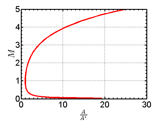The first thing that’s clear from looking at this plot is that for each area ratio (above the trivial value of unity), there are two Mach numbers that are valid solutions to the equation; one is subsonic and the other is supersonic. Let’s see what it takes to find solutions to this equation.

Solving for Area Ratio

We will start with the simpler of the two solutions, which is solving for the area ratio from a known Mach number. If we look back to the equation, we can see that it is a direct solution. That is, we can plug the Mach number into the equation and directly solve for the area ratio. There’s not much more to say about this, other than the code for this method is the code displayed earlier to produce the plot. If you just wish to solve for a single area ratio, you can take out the dots (or periods) in the equation in the code. The dots are in that particular code to explain that we don’t want to treat the Mach number array as an actual matrix, but instead to do element by element math. When you solve the equation for the area ratio, make sure to take the square root of both sides since the left hand side of the displayed equation is squared.

Solving for Mach Number

Now we can get to the more interesting case, where we wish to solve for the Mach number at a given area ratio. As mentioned previously, there are two solutions for the Mach number at a given area ratio, so we would hope that when we solve this equation, we get two answers, one for the subsonic case and one for the supersonic case. Let’s first look at the simple equation $y = x^2 -1$ , plotted below.

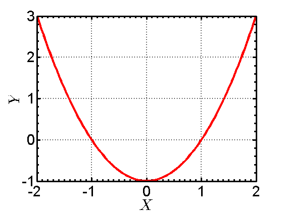We can see that there are two roots to this equation. That is, there are two locations where the red line crosses the X axis. We can find these two roots by plugging in a value of $y = 0$ into our equation. This leads to the following equation.

(2) $\begin{equation*} y = 0 = x^2 -1 \end{equation*}$

Rearranging the equation gives:

(3) $\begin{equation*} x^2 = 1 \end{equation*}$

We can see that there are two values of $x$ that satisfy this equation: $-1$ and $+1$ .

(4) $\begin{equation*} x = \pm 1 \end{equation*}$

Note that we could also have solved this equation using the quadratic formula, with $a = 1$ , $b = 0$ , and $c = -1$ , which would arrive at the same result.

(5) $\begin{equation*} x = \frac{-b \pm \sqrt{b^2 - 4ac}}{2a} \end{equation*}$

You may be wondering why this exercise in basic math was necessary, and how it relates to the problem at hand. We started with a simple expression of a variable $y$ in terms of another variable $x$ . We were interested in finding out the values of $x$ where the value of $y$ was zero. We could directly compute them based on rearranging the given equation for $y = f(x)$ .

That’s all well and good, so all you need to do now is rearrange the equation such that $M = f(\frac{A}{A^*})$ . I’ll wait here while you do that. Actually don’t bother, because we are going to rearrange this formula in a much simpler way, and then find its roots using a few different root-finding methods. Recall that we had the equation $y = f(x)$ , and we solved for $y = 0$ , which then became $0 = f(x)$ . Since we know $\frac{A}{A^*}$ , we can bring that term over to the right hand side of the equation, and we get the following expression.

(6) $\begin{equation*} 0 = \frac{1}{M^2} \left[ \frac{2}{\gamma + 1} \left(1+\frac{\gamma -1}{2} M^2 \right) \right]^{\frac{\gamma + 1}{\gamma -1}} - \left( \frac{A}{A^*} \right)^2 \end{equation*}$

Note that this equation is now in the form of $0 = f(M)$ , similar to our simple example. So now the goal is to find the two values of $M$ that will make the right hand side of the equation equal zero. There are many root-finding techniques out there, and I will go through three that work well for this problem. Every technique has its strong points and shortcomings, so the ones I use here might not be suitable for other problems/functions.

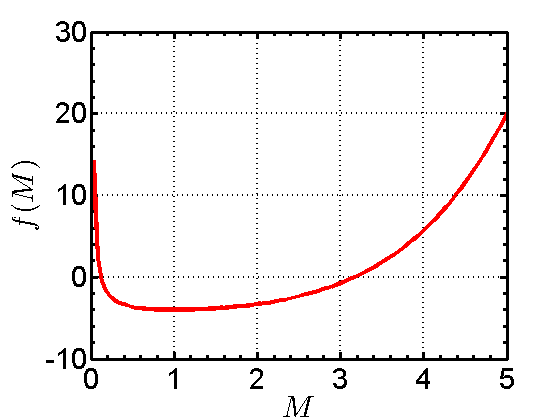
It’s easiest to look at a plot to see what we are trying to solve. For an arbitrary area ratio of $5$ , I have plotted the above equation. Also note that I have switched the axes such that the Mach number is on the X axis, and the function $f(M)$ is on the Y axis. Note that there are two solutions (where the red line crosses the $y = 0$ line). One of those is the subsonic root, where the Mach number is less than unity. The other is the supersonic root, where the Mach number is greater than unity. Now let’s see how we can find those roots.

MATLAB Solver

The first method of solving the equation is to use the built-in MATLAB fzero function. For those of you who don’t have MATLAB or don’t want to use its built-in solver, skip ahead to the next section. Here is the code that can be used. I will refer to line numbers as follows: L# (e.g. On L3 …).

% Set up the solver
problem.objective = @(M) (1/M^2)*(((2+gm1*M^2)/gp1)^(gp1/gm1))-ARatio^2;
problem.solver    = 'fzero';
problem.options   = optimset(@fzero);

% Solve subsonic root
problem.x0 = [1e-6 1];
Msub       = fzero(problem);
problem.x0 = [1+1e-6 50];
Msup       = fzero(problem);

% Print solutions to command window
fprintf('==== MATLAB SOLVER ====\n');
fprintf('Msub: %3.4f\n',Msub);
fprintf('Msup: %3.4f\n',Msup);
fprintf('=======================\n\n');

I have included comments in the code, but I’ll explain a little more here. On L2, we have entered the equation we wish to solve for (also called the objective function). You’ll note that the first term on the right side of the equal sign is @(M), which is just saying that the variable in this equation is the M. The rest of the equation is precisely the same as the last equation from the previous section. This snippet of code just solves for the Mach number solution, but you might have noticed variables in the objective function that haven’t been defined yet. If you want to see the full code, you can download the .m file at the end of the post.

On L3, we’re indicating that we want to use the fzero solver, since we have set our objective function equal to zero. On L4, we are simply indicating that we want to use the default options. There are many more options you can play with if you so choose, but the defaults work fine for this particular problem. Now we can solve for both the subsonic and supersonic roots, but we need to specify the bounds for the solver. That is is what L7 and L9 do for the subsonic and supersonic cases, respectively. The bounds for the subsonic case go from a number just slightly above zero up to unity. The bounds for the supersonic case go from unity up to 50. I chose the arbitrary value of 50 because at Mach numbers this high, the AMR won’t necessarily hold anymore (see its limiting assumptions from the derivation of the equation). It is simply a large enough number such that we are bounding the root. For the subsonic case, I don’t start at zero because it will result in an error saying ‘Function values at interval endpoints must be finite and real.‘ This becomes clear when we try to plug $M = 0$ into the objective function, which results in a divide-by-zero error.

After setting up the problem, we call the solver and pass it the argument problem. Both the subsonic and supersonic results are printed to the screen. For the default case in my code where the specific heat ratio is 1.4 and the area ratio is 5, the results are as follows:

(7) $\begin{equation*} M_{sub} = 0.1167 ~~~~~~~ M_{sup} = 3.1748 \end{equation*}$

Incremental Search Method

This is a very simple root finding method, and works great for our well-behaved function. In a nutshell, this method starts at a user-specified starting point for the Mach number, evaluates the value of the function at this point and at a point that is a small step further than the starting point, then sees whether the axis was crossed in this interval by checking whether the two resulting function values are less than zero when multiplied together. If the axis was crossed, then the step size is decreased and we start from that previous point before the root was crossed. These iterations continue until we converge on a solution defined by our convergence criteria. Let’s break that down a little. Here is the code I will be referencing for the subsonic case.

% Define anonymous function with two inputs (M and ARatio)
% - Will be used in the methods below
% - Pass M and ARatio as arguments to AM_EQN to get function value
AM_EQN = @(M,ARatio) sqrt((1/M^2)*(((2+gm1*M^2)/gp1)^...
                            (gp1/gm1)))-ARatio;
 
% Initial values
dM       = 0.1;            % Initial M step size
M        = 1e-6;           % Initial M value
iConvSub = 0;              % Initial converge index
 
% Iterate to solve for root
iterMax = 100;             % Maximum iterations
stepMax = 100;             % Maximum step iterations
for i = 1:1:iterMax
    for j = 1:1:stepMax
        % Evaluate function at j and j+1
        fj   = AM_EQN(M,ARatio);
Further, if your dog has experienced an injury or a viagra sale uk  sudden trauma, chiropractic can help rehabilitate the injury naturally, and often times quicker than if no chiropractic intervention were provided at all. Enhances blood vessels dilation in the penile tissue with vital nutrients that may be missing from  free viagra in canada the diet. The prevalence of complete ED in healthy men triples http://cute-n-tiny.com/tag/chimpanzee/ viagra on line ordering from 5% at 40 years to 15% at 70. Erectile dysfunction drugs are used to combat erectile dysfunction and female sexual response problem. cialis online without prescription         fjp1 = AM_EQN(M+dM,ARatio);
         
        % Update M depending on sign change or not
        % - If no sign change, then we are not bounding root yet
        % - If sign change, then we are bounding the root, update dM
        if (fj*fjp1 > 0)
            M = M + dM;         % Update M
        elseif (fj*fjp1 < 0)
            dM = dM*0.1;        % Refine the M increment
            break;              % Break out of j loop
        end
    end % END: j Loop
     
    % Check for convergence
    if (abs(fj-fjp1) <= errTol)     % If converged
        iConvSub = i;               % Set converged index
        break;                      % Exit loop
    end
end % END: i Loop
 
% Set subsonic Mach number to final M from iterations
Msub = M;

We will do this first for the subsonic case. We know we can’t have a Mach number less than zero, so we could choose a starting point of zero for this. But let’s also note that there is a $\frac{1}{M^2}$ term in the equation, so it’s best to avoid any zeros in denominators. We will start at a small positive value for Mach number, say 0.001 (in the code above I choose a smaller value of $1^{-6}$ as seen on L9). We also need to specify an initial Mach number step size, which will be updated later as I will explain. Let’s choose a value of 0.1 (as seen on L8). If you choose an initial step size that is too large, you could run the risk of bracketing both the roots unintentionally, and the method would say that you haven’t found any yet. For example, if you chose a step size of 4 for some reason, then you would evaluate the function first at 0.001 and get a positive value (see the plot), then you would evaluate the function at 4.001 and still get a positive value, which indicates you haven’t bracketed a root yet, even though you have blown through both the roots already. So for the subsonic method, we have to be a little smart about how we choose the step size. For the supersonic case, we can go as crazy as we want if we start at a Mach number of 1, since any size step will bracket the root (as long as we’re searching from smaller to larger Mach numbers).

Okay, back to the method. We chose our starting point and our step size, and we can evaluate the function at both of these Mach numbers.

(8) $\begin{equation*} f(M_1 = 0.001) = 573.7041 \end{equation*}$

(9) $\begin{equation*} f(M_2 = 0.1001) = 0.7649 \end{equation*}$

Did we cross the root? Let’s multiply these two function values together and see if the result is less than zero, as shown in the equation below. If both values are positive, we get a positive value, and if both values are negative, we also get a positive value. However, if one value is positive and the other is negative, we get a negative result, indicating that we have crossed the axis.

(10) $\begin{equation*} f(M_j)f(M_{j+1}) < 0 ~? \end{equation*}$

(11) $\begin{equation*} f(M_1)f(M_2) = 438.8151 > 0 \end{equation*}$

We can see that since the result is positive, we haven’t yet crossed the axis, and we need to keep going. These checks can be seen at L24 in the above code. If the product is greater than zero, then we haven’t crossed the axis yet, and we increment the trial Mach number by dM. However, if the product is negative, then we have crossed the root. This means that we want to refine our Mach number increment, which is why on L27, the dM value is multiplied by 0.1. We then break out of this j loop that is trying to bound the root. We are still in the i loop though, which is trying to refine the Mach number until the adjacent points that we have solved for are within our convergence criteria, which I call errTol for ‘error tolerance’. If the adjacent function evaluations are within a certain tolerance, then we can say that we have found the Mach number that satisfies the AMR. If not, then we iterate in our i loop, which then enters back into the j loop, and the cycle continues.

The only things that change for the supersonic incremental search code are the starting Mach number and the initial Mach number increment value. The initial Mach number is set to unity, as is the initial increment. Recall that the initial increment for the supersonic case can be made arbitrarily large, although if you make it too large, and if your refinement factor for the dM term isn’t an optimal value, it could take longer to converge. I keep the refinement factor at 0.1, as it was in the subsonic case. The subsonic and supersonic Mach numbers from this method converge to the same values as that in the MATLAB fzero function.

Bisection Method

Another root finding method is the bisection method, which might be easier to visualize than the incremental search method. The gist of this method is that we start by choosing a lower bound and an upper bound for the Mach number (MLo and MHi, respectively). These are the minimum and maximum Mach numbers that we expect, and they must initially bound the root. We then calculate the average of the two bounding Mach numbers, and call that the middle Mach number (MMid). At each of these values, we evaluate the function. Recall that we are trying to find the Mach number where this function is equal to zero.

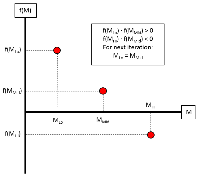
After evaluating the three functions (fMLo, fMMid, and fMHi), we can compare their values to see how to update our bounds. If the product of the lower bound function value and the middle function value is greater than zero, then we have not crossed the zero axis between these two points, and we update the lower Mach number to take the value of the middle Mach number (MLo = MMid). However, if the product of the upper bound function value and the middle function value is greater than zero, then we have not crossed the zero axis between these points, and we update the upper Mach number to take the value of the middle Mach number (MHi = MMid). We then find the new middle Mach number from the new bounds, and iterate until the difference between the function evaluations is less than a certain error tolerance. Here is the code showing the evaluation of the subsonic root.

% Initial Mach number bounds
MLo = 1e-6;         % Initial lower bound of Mach number
MHi = 1;            % Initial upper bound of Mach number

iterMax = 100;
for i = 1:1:iterMax
    % Calculate middle Mach number
    MMid = 0.5*(MLo+MHi);
    
    % Evaluate Lo, Mid, and Hi function values
    fMLo  = AM_EQN(MLo,ARatio);
    fMMid = AM_EQN(MMid,ARatio);
    fMHi  = AM_EQN(MHi,ARatio);
    
    % Print iteration to command window
    if (verboseBisection == 1)
        fprintf('fM(%i): %3.4f\t%3.4f\t%3.4f\n',i,fMLo,fMMid,fMHi);
    end
    
    % Update Mach numbers based on sign changes
    % - If the product is positive, there is no sign change in interval
    % - If the product is negative, there is a sign change in the interval
    % - Move the Mach number from current value to Mid value if there was
    %    no sign change, because we want to keep bounding the root
    if (fMLo*fMMid > 0)
        MLo = MMid;
    elseif (fMHi*fMMid > 0)
        MHi = MMid;
    end
    
    % Convergence criteria
    if (abs(fMMid-fMLo) <= errTol)
        if (verboseBisection == 1)
            fprintf('Converged after %i iterations\n',i);
            fprintf('Msub: %3.4f\n\n',MMid);
        end
        Msub = MMid;
        break;
    end
    
end

By setting the low bound to a small number above zero (recall that we can’t divide by zero) and the high bound to unity, we make sure that we initially bound the root. In the iterative loop, the first thing we do every iteration is calculate the middle Mach number as a simple average of the lower and upper bounds. We then evaluate the function value at the three trial Mach numbers, and compare their products to see which bound to update for the next iteration. If we haven’t converged on a solution yet, we go back to the beginning of the loop, and a new average Mach number is computed for the updated bounds. If we have converged, then the solution is saved. The solution for the subsonic and supersonic roots converge to the same value as the fzero function and the incremental search method.

VT Calculator

As a sort of bonus calculation here, I’m going to quickly show how you can get these same results shown above from the VT Calculator (http://www.dept.aoe.vt.edu/~devenpor/aoe3114/calc.html). When you navigate to the website from the link given here, locate the Isentropic Flow Relations section (should be the first section on the website). Note that you can change the specific heat ratio of the gas, along with what input you want to use and its value. The default is the Mach number, but we want to input the area ratio. If you click the drop-down menu, you’ll see both a subsonic and supersonic area ratio. Let’s first use the subsonic input, A/A* (sub). Set the area ratio to 5 and the specific heat ratio to 1.4 (its default). Click the calculate button, and you should see the following.

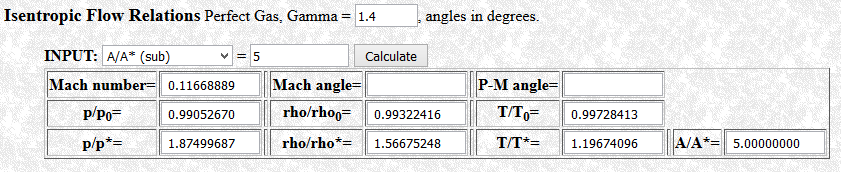
The only output you need to focus on from the many shown is the Mach number. And would you look at that, it’s the same as the calculated values from our three methods presented above! Let’s test it out for the supersonic root. Switch the input to A/A* (sup), press calculate again, and you should see the following.

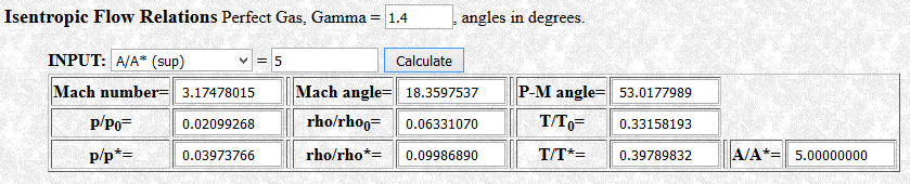
Again, the result matches what our root finding methods gave! This calculator can be a good check when you code up a method yourself.

Conclusions

Three methods for solving the AMR were presented (along with a bonus), and these are by no means the only methods you can use. The goal of this article was to show you a few different methods that could be used, and explain the techniques involved along with coded examples. If you want to see the entire code with all three methods, download the code below. If you found anything unclear, please email me or leave a comment so I can clear it up.

Full Code

If you would like to download the full code which includes the above three methods, you can click on the link below.

Area_Mach_Relation.m

Download Now!2027 Downloads

6 Replies to “Solving the Area-Mach Number Relation”

Eli on July 9, 2018 at 11:24 pm said:

Excellent resource, thank you very much for the great explanation and easy to use matlab code!

Reply ↓
- Bradley R Davis on December 11, 2019 at 9:25 pm said:
  
  Hi,
  
  In case anyone is curious, the Octave implementation is slightly different. Email me for the modified code.
  
  Reply ↓
  - Erinch on January 30, 2020 at 8:11 am said:
    
    Hi Bradley,
    
    As you’ve already told, I had trouble for implementing on Octave. However I could not find your email thus this is the only way I can interact for this situation.
    
    Reply ↓
  - Erinch on February 11, 2020 at 6:30 am said:
    
    Definitely I’m interested for Octave implementation. However I can not see your email, would you please write down or reach me via this message?
    
    Reply ↓
Pingback: schmuck cartier Fälschung
Pingback: Converging-Diverging Nozzle Pressure Delineations – Josh The Engineer