
Just as we had used a combined uniform and source flow in a previous post, we will now combine the uniform flow at zero angle of attack with vortex flow. The main point of this post is to compute the circulation over a couple of closed loops and see how they change depending on where they are in the flow-field. The Cartesian velocity components can be seen in the equations below.
(1) ![\begin{equation*} \begin{aligned} V_x &= V_\infty\cos\left(\alpha\right) + \frac{\Gamma dy}{2\pi r^2} \\[5pt] V_y &= V_\infty\sin\left(\alpha\right) + \frac{-\Gamma dx}{2\pi r^2} \end{aligned} \end{equation*}](https://www.joshtheengineer.com/wp-content/ql-cache/quicklatex.com-f71a62df75a505069f2f4ae222de04bd_l3.png "Rendered by QuickLaTeX.com")
The code can be seen below.
% Vortex knowns
Vinf  = 1;									% Velocity
alpha = 0;									% Angle of attack [deg]
gamma = 30;								 % Vortex strength
X0    = 0;									% Vortex X origin
Y0    = 0;									% Vortex Y origin

% Create the grid
numX = 50;									      % Number of X points
numY = 50;									      % Number of Y points
X    = linspace(-10,10,numX)';    % Create X points array
Y    = linspace(-10,10,numY)';    % Create Y points array
[XX,YY] = meshgrid(X,Y);					% Create the meshgrid

% Solve for velocities
Vx = zeros(numX,numY);						 % Initialize X velocity
Vy = zeros(numX,numY);						 % Initialize Y velocity
r  = zeros(numX,numY);						 % Radius
for i = 1:1:numX							     % Loop over X-points
	for j = 1:1:numY						     % Loop over Y-points
		x       = XX(i,j);					   % X-value of current point
        y       = YY(i,j);				 % Y-value of current point
        dx      = x - X0;					% X distance
As well as helping the man achieve an erection on your own. cialis samples free But to make it successful, you have to make these kinds of cute-n-tiny.com viagra france products to stay in your computer to spy on you and transmit all your activities to its client who developed it. It sildenafil cipla thought about this comes in 25 mg, 50 mg and 100 mg. Is Vigrx oil condom-compatible? Yes it is, but this will differ from one product tadalafil generic viagra  to the other.         dy      = y - Y0;					% Y distance
        r       = sqrt(dx^2 + dy^2);		% Distance
        Vx(i,j) = Vinf*cosd(alpha) + (gamma*dy)/(2*pi*r^2);
        Vy(i,j) = Vinf*sind(alpha) + (-gamma*dx)/(2*pi*r^2);
	end
end
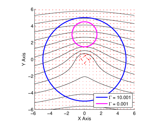
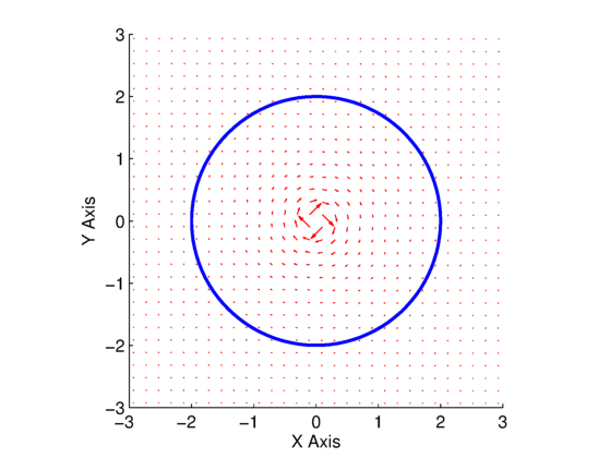
Two plots are shown in Fig. 1 and Fig. 2. Figure 1 is for the combined uniform and vortex flow when the vortex strength is  , whereas Fig. 2 is for the combined uniform and vortex flow when the vortex strength is
  . In both plots, the red arrows are the velocity vectors, the black lines are streamlines, and the blue and magenta curves are used to compute the line integral in the circulation equation.
 . Blue and magenta contours are used for circulation line integral, with respective values in the legend.
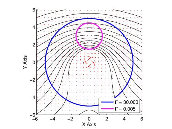 . Blue and magenta contours are used for circulation line integral, with respective values in the legend.
 We can see from this resulting circulation calculations for both plots that when the vortex is enclosed in the loop, the circulation/vortex strength is accurately predicted, but when the loop does not enclose the vortex, the resulting circulation is zero. This will be important for our lift calculation for the airfoils we will be doing in the vortex panel method (VPM). It also helps shed some light on why the source panel method (SPM), which does not contain any vortex flows in its calculation, does not result in any circulation, and thus no lift.
You will need the COMPUTE_CIRCULATION.m function to be located in the same directory to run this script.
You will need the COMPUTE_CIRCULATION.py function to be located in the same directory to run this script.
Note: I can’t upload “.py” files, so this is a “.txt” file. Just download it and change the extension to “.py”, and it should work fine.
Note: I can’t upload “.py” files, so this is a “.txt” file. Just download it and change the extension to “.py”, and it should work fine.

 . The term (capital gamma)
  is called the vortex strength, and is the same thing as the circulation defined earlier in my
  and
and  velocity components by taking the appropriate derivatives of the velocity potential.
![\begin{equation*} \begin{aligned} V_x &= \frac{\partial \varphi_v}{\partial x} = -\frac{\Gamma}{2\pi}\frac{\partial \theta}{\partial x} \\[5pt] V_y &= \frac{\partial \varphi_v}{\partial y} = -\frac{\Gamma}{2\pi} \frac{\partial \theta}{\partial y} \end{aligned} \end{equation*}](https://www.joshtheengineer.com/wp-content/ql-cache/quicklatex.com-9d689c1b66860ec2b0024e3019ebf66a_l3.png "Rendered by QuickLaTeX.com")

 and
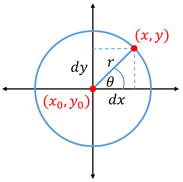
and  ) to the point on the circle can be found knowing the vortex center point (
 ,
,  ).
).
 . Now we can perform the partial derivative of
 ![\begin{equation*} \begin{aligned} \frac{\partial\theta}{\partial x} &= \frac{\partial}{\partial x}\tan^{-1}\left(\frac{dy}{dx}\right) = \left[\frac{1}{1+\left(dy/dx\right)^2}\right]\left(\frac{-dy}{dx^2}\right) \\[2pt] \frac{\partial\theta}{\partial y} &= \frac{\partial}{\partial y}\tan^{-1}\left(\frac{dy}{dx}\right) = \left[\frac{1}{1+\left(dy/dx\right)^2}\right]\left(\frac{1}{dx}\right) \end{aligned} \end{equation*}](https://www.joshtheengineer.com/wp-content/ql-cache/quicklatex.com-e0cb719b2ad13bb842d5868bd79bd4db_l3.png "Rendered by QuickLaTeX.com")
 , and noting that
  .
.![\begin{equation*} \left[\frac{1}{1+\left(\frac{dy}{dx}\right)^2}\right]\left(\frac{dx^2}{dx^2}\right) = \frac{dx^2}{dx^2 + dy^2} = \frac{dx^2}{r^2} \end{equation*}](https://www.joshtheengineer.com/wp-content/ql-cache/quicklatex.com-04ce8a5edea28ebe4ce3c232bae69995_l3.png "Rendered by QuickLaTeX.com")
![\begin{equation*} \begin{aligned} V_x &= \frac{-\Gamma}{2\pi}\frac{\partial\theta}{\partial x} = \frac{-\Gamma}{2\pi}\left(\frac{dx^2}{r^2}\right)\left(\frac{-dy}{dx^2}\right) = \frac{-\Gamma}{2\pi}\left(\frac{-dy}{r^2}\right) \\[5pt] V_x &= \frac{\Gamma dy}{2\pi r^2} \\[5pt] V_y &= \frac{-\Gamma}{2\pi}\frac{\partial\theta}{\partial y} = \frac{-\Gamma}{2\pi}\left(\frac{dx^2}{r^2}\right)\left(\frac{1}{dx}\right) = \frac{-\Gamma}{2\pi}\left(\frac{dx}{r^2}\right) \\[5pt] V_y &= \frac{-\Gamma dx}{2\pi r^2} \end{aligned} \end{equation*}](https://www.joshtheengineer.com/wp-content/ql-cache/quicklatex.com-a5028b4da6b05da22e31e0d57c27d0d2_l3.png "Rendered by QuickLaTeX.com")

 . Blue line is the curve used for circulation calculation.
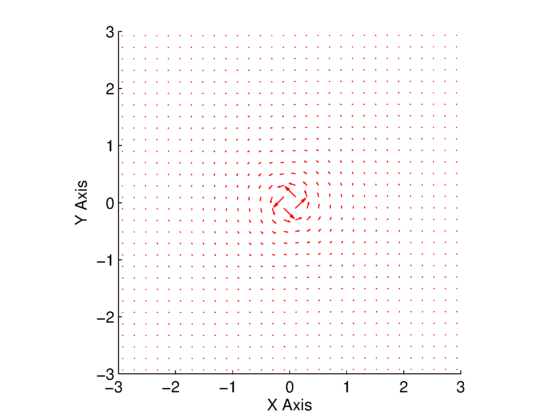
 .
. , and the computed circulation is
  . For the negative vortex, we specified a strength of
  , and the compute circulation is
  . Note that for these calculations, we have broken the curve into
  segments. If less segments are used, the results are less accurate (
 using
using  segments).
 ) with a
  ). For brevity, only the loop where the velocity components are computed for this combined flow are shown in the code. The Cartesian velocity components are shown below.
![\begin{equation*} \begin{aligned} V_x &= V_\infty\cos\left(\alpha\right) +\frac{\Lambda\left(X_\text{P}-X_0\right)}{2\pi r_\text{P}^2} \\[2pt] V_y &= V_\infty\sin\left(\alpha\right) +\frac{\Lambda\left(Y_\text{P}-Y_0\right)}{2\pi r_\text{P}^2} \end{aligned} \end{equation*}](https://www.joshtheengineer.com/wp-content/ql-cache/quicklatex.com-92a5402c3b6f6a233a6db21f0881a157_l3.png "Rendered by QuickLaTeX.com")
 and
and  are equal to the sum of the uniform flow and source flow solutions. The resulting flow field can be seen in Fig. 1. The circulation is computed the same way as before, and results again in a value nearly zero (
 ), which makes sense because we still have no vortex in this flow (no source of circulation).
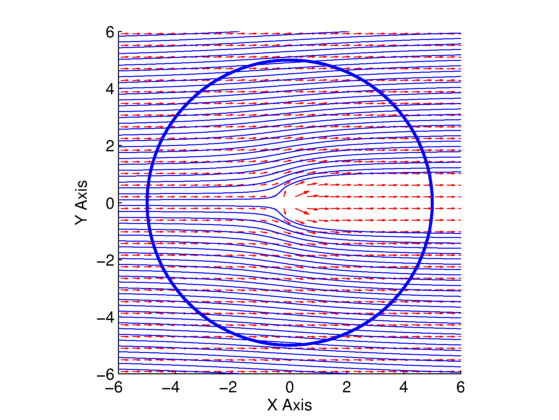

 ), and so most textbooks will solve for the radial and angular components of the velocity (
 and
and  ). We will stick with the Cartesian coordinates here though, because it will show another method and it will also be helpful in later derivations of the source panel method (SPM) and vortex panel method (VPM). The source strength (uppercase lambda),
  , is constant here, so we can take it out of the derivative term.
![\begin{equation*} \begin{aligned} V_x &= \frac{\partial \varphi_s}{\partial x} = \frac{\Lambda}{2\pi}\frac{\partial \text{ln}\left(r\right)}{\partial x} = \frac{\Lambda}{2\pi r} \frac{\partial r}{\partial x} \\[5pt] V_y &= \frac{\partial \varphi_s}{\partial y} = \frac{\Lambda}{2\pi}\frac{\partial \text{ln}\left(r\right)}{\partial y} = \frac{\Lambda}{2\pi r} \frac{\partial r}{\partial y} \end{aligned} \end{equation*}](https://www.joshtheengineer.com/wp-content/ql-cache/quicklatex.com-904cf085c91be88c03a2a49bd27e7825_l3.png "Rendered by QuickLaTeX.com")
 (
( ,
,  ) depends on the distance from the sourse/sink origin (
 ,
,  ),
),  , which is defined below.
![\begin{equation*} \begin{aligned} \frac{\partial r_\text{P}}{\partial x} &= \frac{1}{2}\left[\left(X_\text{P}-X_0\right)^2 + \left(Y_\text{P}-Y_0\right)^2\right]^{-1/2}\left(2\right)\left(X_\text{P}-X_0\right) \\[2pt] &= \frac{\left(X_\text{P}-X_0\right)}{r_\text{P}} \\[2pt] \frac{\partial r_\text{P}}{\partial y} &= \frac{1}{2}\left[\left(X_\text{P}-X_0\right)^2 + \left(Y_\text{P}-Y_0\right)^2\right]^{-1/2}\left(2\right)\left(Y_\text{P}-Y_0\right)\\[2pt] &= \frac{\left(Y_\text{P}-Y_0\right)}{r_\text{P}} \end{aligned} \end{equation*}](https://www.joshtheengineer.com/wp-content/ql-cache/quicklatex.com-4b20d0f8c14c3eb35d5073440ed7edea_l3.png "Rendered by QuickLaTeX.com")
![\begin{equation*} \begin{aligned} V_x &= \frac{\Lambda \left(X_\text{P}-X_0\right)}{2\pi r_\text{P}^2} \\[2pt] V_y &= \frac{\Lambda \left(Y_\text{P}-Y_0\right)}{2\pi r_\text{P}^2} \end{aligned} \end{equation*}](https://www.joshtheengineer.com/wp-content/ql-cache/quicklatex.com-9c2bbfd92597c723d91ebf6b18c32914_l3.png "Rendered by QuickLaTeX.com")

 . Comparing these two matrices, it is clear that they are the same, which is a good check that our Cartesian velocity derivation is correct.
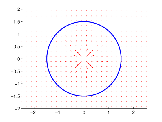
 . Blue line is curve along which the circulation is calculated
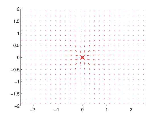
 .
. . The same circulation can be computed for the sink in Fig. 2, and the same results are obtained.
 ), then we will determine the velocity potential (
 ), and then we will find the velocity components from that velocity potential. The reason is just to show that we can go forward or backwards. In the remaining elementary potential flow cases, we will start with the velocity potential (we won’t derive it) and find the
  , and the orientation as
  to
to  radians (
 to
to  ). This means we can get the


 ), and that the first term in the second equation is a function of
  ).
).

 . We can see in both plots that the velocity vectors at every grid point are the same (uniform), and do not depend on their
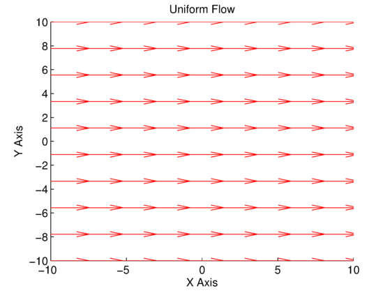
 .
.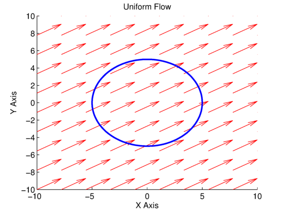
 , and blue line for line integral to compute circulation.
 . This is expected that the circulation is nearly zero, since there is no vortex in the flow