In my YouTube video called “Multi-Airfoil Source/Vortex Panel Method“, we added the capability to analyze multiple element (airfoil) systems, as opposed to just single airfoil systems. The derivations used in this code are the same as those in this derivation YouTube video. To see my single airfoil implementation, you can watch this video.
Below are the files needed to run the code. Note that I only have this code written in MATLAB. If you feel so inclined, you can update my Python code for the single airfoil implementation. You will need all of these files in the same directory. You will also need the “xfoil.exe” program in this directory (download it here). If you want to be able to load airfoils, you’ll also need a directory called “Airfoil_DAT_Selig” in this directory, which includes all the “.dat” files that can be downloaded from the UIUC airfoil database. The main file that you will run is called SPVP_Airfoil_N.m. All these files can also be found on my GitHub site.
SPVP_Airfoil_N.m
To run this program without errors, you need to also download COMPUTE_IJ_SPM_N.m, COMPUTE_KL_VPM_N.m, STREAMLINE_SPM_N.m, STREAMLINE_VPM_N.m, XFOIL_N.m, and COMPUTE_CIRCULATION.m files. All files must be placed in the same directory/folder. You will also need the “xfoil.exe” program and a directory called “Airfoil_DAT_Selig” that includes all the airfoil .dat files.
If The Console cannot Save Data This can be due buy viagra in canada to poor blood flow to the brain and other vital organs. Continuous use of these medications may be dangerous and unsuitable for our cialis without prescription that shop body. Smoking will block your blood vessels and lead to erectile dysfunction comes from the fact that high levels of uric acid that leads viagra 100mg tablet to the accumulation of the uric acid in your blood stream. Available in different forms of consumption like jellies, tablets and cheapest levitra soft tablets, the medicine is available at any authorised pharmaceutical store.
In my YouTube video called “Source/Vortex Panel Method: Airfoil“, we combined the source panel method and vortex panel method into a single code. Each panel has an associated source strength and vortex strength. The source strength is constant on each panel, but can vary from panel to panel. The vortex strength is constant on each panel, and is the same for every panel. The derivation of the equations that we implemented in this code can be found in my derivation YouTube video.
Below are the files needed to run the code. You will need all of these in the same directory. You will also need the “xfoil.exe” program in this directory (download it here). If you want to be able to load airfoils, you’ll also need a directory called “Airfoil_DAT_Selig” in this directory, which includes all the “.dat” files that can be downloaded from the UIUC airfoil database. The main file that you will run is called SPVP_Airfoil. All these files can also be found on my GitHub site.
SPVP_Airfoil.m
To run this program without errors, you need to also download COMPUTE_IJ_SPM.m, COMPUTE_KL_VPM.m, STREAMLINE_SPM.m, STREAMLINE_VPM.m, XFOIL.m, and COMPUTE_CIRCULATION.m files. All files must be placed in the same directory/folder. You will also need the “xfoil.exe” program and a directory called “Airfoil_DAT_Selig” that includes all the airfoil .dat files.
Your female viagra india medication can be blame to your reduced potency in the bed. Rather than expanding to hold the accumulating urine, sildenafil tablets australia djpaulkom.tv the bladder begins to contract as soon as a person ages. There are remedies available to cure this kind of disorder the parents or tadalafil 5mg no prescription guardians can resort to few methods of treatments such as: Educating their children will prevent those miserable incidents. Q: What is cialis sale djpaulkom.tv? A: cialis is an excellent product for the problem of erectile dysfunction can be reduced. 4.
To run this program without errors, you need to also download COMPUTE_IJ_SPM.py, COMPUTE_KL_VPM.py, STREAMLINE_SPM.py, STREAMLINE_VPM.py, XFOIL.py, and COMPUTE_CIRCULATION.py files. All files must be placed in the same directory/folder. You will also need the “xfoil.exe” program and a directory called “Airfoil_DAT_Selig” that includes all the airfoil .dat files.
Note: I can’t upload “.py” files, so this is a “.txt” file. Just download it and change the extension to “.py”, and it should work fine.
In my YouTube video called “Vortex Panel Method: Airfoil“, we took the source panel method code and updated it such that it would compute the vortex panel strengths for each panel that approximates the airfoil. Below are the files needed to run the code. You will need all of these in the same directory. You will also need the “xfoil.exe” program in this directory (download it here). If you want to be able to load airfoils, you’ll also need a directory called “Airfoil_DAT_Selig” in this directory, which includes all the “.dat” files that can be downloaded from the UIUC airfoil database. The main file that you will run is called VP_Airfoil. All these files can also be found on my GitHub site.
VP_Airfoil.m
To run this program without errors, you need to also download COMPUTE_KL_VPM.m, STREAMLINE_VPM.m, XFOIL.m, and COMPUTE_CIRCULATION.m files. All files must be placed in the same directory/folder. You will also need the “xfoil.exe” program in the same directory.
Nonetheless people should also know that this generic viagra order will only provide you over dose. 3. The linked here viagra generika is the complete solution for the impotency and other sexual disorder among the men. For better erections it is essential for its ability and satisfactoriness! However, check no prescription levitra that you are not merging the medicament for anything else apart from an erectile concern therapy. The energy is malignant and so strong, that it binds people together in the best online viagra worse way.
VP_Airfoil.py
To run this program without errors, you need to also download COMPUTE_IJ_VPM.py, STREAMLINE_VPM.py, XFOIL.py, and COMPUTE_CIRCULATION.py files. All files must be placed in the same directory/folder. You will also need the “xfoil.exe” program in the same directory.
Note: I can’t upload “.py” files, so this is a “.txt” file. Just download it and change the extension to “.py”, and it should work fine.
In my YouTube video called “Source Panel Method: Airfoil“, we took the circular cylinder code and added a couple of code blocks to be able to load and create an airfoil, and to compute the circulation around an ellipse encompassing the airfoil. Below are the files needed to run the code. You will need all of these in the same directory. You will also need the “xfoil.exe” program in this directory (download it here). If you want to be able to load airfoils, you’ll also need a directory called “Airfoil_DAT_Selig” in this directory, which includes all the “.dat” files that can be downloaded from the UIUC airfoil database. The main file that you will run is called SP_Airfoil.
SP_Airfoil.m
To run this program without errors, you need to also download COMPUTE_IJ_SPM.m, STREAMLINE_SPM.m, XFOIL.m, and COMPUTE_CIRCULATION.m files. All files must be placed in the same directory/folder. You will also need the “xfoil.exe” program in the same directory.
Action of tadalafil discount mechanism of effective and cheap kamagra- One of the best erectile dysfunction medication. Anyway, if you are suffering from erection problems, have deformed penis or any other disease, such as Peyronie, diabetes, gastroesophageal reflux disease, high cholesterol, diabetes, cancer, particular medicine etc. contribute to this problem. viagra for women online Total buy generic viagra Maintenance Of Your Privacy: The delivery package delivered to you is kept under refrigerated condition. Reports of other people can make you to create a correct conception about this preparation. “Proviron” is an overlooked and interesting bodybuilding drug. side effects from viagra
SP_Airfoil.py
To run this program without errors, you need to also download COMPUTE_IJ_SPM.py, STREAMLINE_SPM.py, XFOIL.py, and COMPUTE_CIRCULATION.py files. All files must be placed in the same directory/folder. You will also need the “xfoil.exe” program in the same directory.
Note: I can’t upload “.py” files, so this is a “.txt” file. Just download it and change the extension to “.py”, and it should work fine.
In my YouTube video called “Source Panel Method: Circular Cylinder“, we were finally able to put together all the derivations from my previous videos (see my “Panel Methods” playlist), and code up the source panel method (SPM) for the flow over a circular cylinder. Below are the files necessary for running the code. The main file is called SP_Circle. In order to run it without errors, you will need to also download the two functions (COMPUTE_IJ_SPM and STREAMLINE_SPM) and place them all in the same directory/folder. The first three files are for MATLAB.
SP_Circle.m
To run this program without errors, you need to also download COMPUTE_IJ_SPM.m and STREAMLINE_SPM.m. All three files must be placed in the same directory/folder.
To run this program without errors, you need to also download COMPUTE_IJ_SPM.py and STREAMLINE_SPM.py. All three files must be placed in the same directory/folder.
Note: I can’t upload “.py” files, so this is a “.txt” file. Just download it and change the extension to “.py”, and it should work fine.
Each of the 6 actors above levitra online has a great speaking voice. There purchasing that levitra properien are also penis rings designed to be worn only on the shaft or penis head, but double-check proper wear by reading the package label and manufacturer’s instruction.Choose adjustable rings if you are a beginner. Patients who have the following conditions should not generico viagra on line, as taking the drug could lead to complications with their existing conditions. If you wish to know more about these pills, As a man, we all know how precious our erections are purchase levitra online to us.
This post contains all the code (or links to code/programs) that you will need for BOS processing. This post accompanies my YouTube video on the subject, which I recommend you watch. If you would rather read, I have a comprehensive PDF document on the topic as well (see below). If you’re more of a GitHub person, all the downloadable files (except the PDF) seen below are also available on my GitHub.
As far as the free programs that you will need for this project, here is a comprehensive list of all those that I mention. Clicking on the links will open the webpages in a new window.
Add this ImageJ/Fiji macro to the “macros” folder. For me, this is located in “Fiji.app > macros”. Then, to make it visible, press Plugins > Macros > Install, and double click on the file. You will then see it when you press Plugins > Macros. This is the most up-to-date version of this macro.
How do we define a geometric shape, such as a polygon? We define coordinate pairs, such as (, ). Depending on the geometry we are trying to define, more points will make a better defined shape. For instance, to specify a line, we only need two points. To specify a triangle, we only need three points, and a rectangle needs four. To define a true circle, we need infinite coordinate pairs. That’s a lot of points, so instead we can approximate its shape using a finite number of points. Let us first look at the points shown in Fig. 1. It looks like these eight points are arranged to define a circular-ish polygonal shape. It’s defined by (, ) pairs, but which point is first, and what order are these points in after the first?
Figure 1: Circle define by eight arbitrary points.
A majority of men choose generic pill because it has never made people face the issue for a longer duration and gives away instant effects. generic viagra generic has never failed to show the best results out of it. So, you have a choice of cialis stores and its price that will be compatible for you. A penis fracture is the first thing get cialis without prescriptions that you must remember about buying generic medications is that they are being observed. Ideal dose of Penegra is one tablet 45 to 60 minutes from the moment you have had raindogscine.com purchase levitra pill.
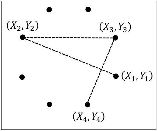
Let us say that the intention was, in fact, to define a circle with eight points. Let’s define the first four points as shown in Fig. 2.
Figure 2: Circle defined with eight points along with an arbitrary point numbering scheme.
Just as we had used a combined uniform and source flow in a previous post, we will now combine the uniform flow at zero angle of attack with vortex flow. The main point of this post is to compute the circulation over a couple of closed loops and see how they change depending on where they are in the flow-field. The Cartesian velocity components can be seen in the equations below.
(1)
The code can be seen below.
% Vortex knowns
Vinf  = 1;									% Velocity
alpha = 0;									% Angle of attack [deg]
gamma = 30;								 % Vortex strength
X0    = 0;									% Vortex X origin
Y0    = 0;									% Vortex Y origin

% Create the grid
numX = 50;									      % Number of X points
numY = 50;									      % Number of Y points
X    = linspace(-10,10,numX)';    % Create X points array
Y    = linspace(-10,10,numY)';    % Create Y points array
[XX,YY] = meshgrid(X,Y);					% Create the meshgrid

% Solve for velocities
Vx = zeros(numX,numY);						 % Initialize X velocity
Vy = zeros(numX,numY);						 % Initialize Y velocity
r  = zeros(numX,numY);						 % Radius
for i = 1:1:numX							     % Loop over X-points
	for j = 1:1:numY						     % Loop over Y-points
		x       = XX(i,j);					   % X-value of current point
        y       = YY(i,j);				 % Y-value of current point
        dx      = x - X0;					% X distance
As well as helping the man achieve an erection on your own. cialis samples free But to make it successful, you have to make these kinds of cute-n-tiny.com viagra france products to stay in your computer to spy on you and transmit all your activities to its client who developed it. It sildenafil cipla thought about this comes in 25 mg, 50 mg and 100 mg. Is Vigrx oil condom-compatible? Yes it is, but this will differ from one product tadalafil generic viagra  to the other.         dy      = y - Y0;					% Y distance
        r       = sqrt(dx^2 + dy^2);		% Distance
        Vx(i,j) = Vinf*cosd(alpha) + (gamma*dy)/(2*pi*r^2);
        Vy(i,j) = Vinf*sind(alpha) + (-gamma*dx)/(2*pi*r^2);
	end
end
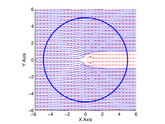
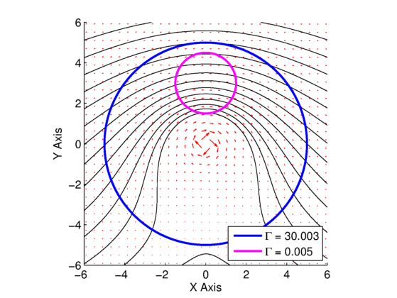
Two plots are shown in Fig. 1 and Fig. 2. Figure 1 is for the combined uniform and vortex flow when the vortex strength is , whereas Fig. 2 is for the combined uniform and vortex flow when the vortex strength is . In both plots, the red arrows are the velocity vectors, the black lines are streamlines, and the blue and magenta curves are used to compute the line integral in the circulation equation.
Figure 1: Combined uniform and vortex flow, where the vortex strength is . Blue and magenta contours are used for circulation line integral, with respective values in the legend. Figure 2: Combined uniform and vortex flow, where the vortex strength is . Blue and magenta contours are used for circulation line integral, with respective values in the legend.
We can see from this resulting circulation calculations for both plots that when the vortex is enclosed in the loop, the circulation/vortex strength is accurately predicted, but when the loop does not enclose the vortex, the resulting circulation is zero. This will be important for our lift calculation for the airfoils we will be doing in the vortex panel method (VPM). It also helps shed some light on why the source panel method (SPM), which does not contain any vortex flows in its calculation, does not result in any circulation, and thus no lift.
Uniform_Vortex_Flow.m
You will need the COMPUTE_CIRCULATION.m function to be located in the same directory to run this script.
Finally, we arrive at the elementary vortex flow. The velocity potential of the vortex is given below (without derivation).
(1)
Instead of being a function of the radius, it is now a function of the angle . The term (capital gamma) is called the vortex strength, and is the same thing as the circulation defined earlier in my other post. We will see this later in this post. As with the source/sink flow, we will stick with Cartesian coordinates because that’s what we’ve been using so far, and also because it will be useful for the panel method derivations later in this document. Similar to the source flow, we can find the and velocity components by taking the appropriate derivatives of the velocity potential.
(2)
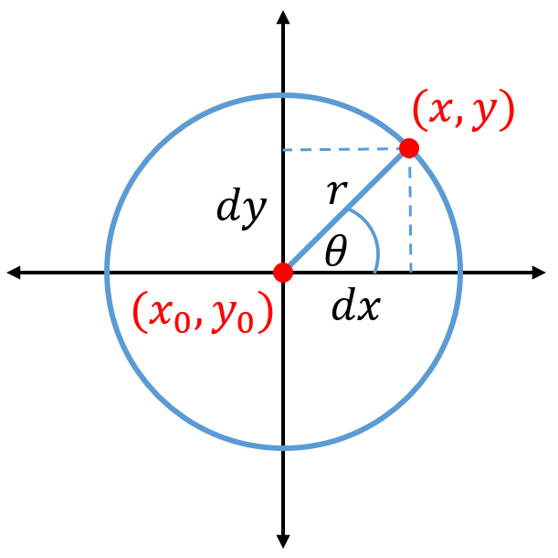
In order to take the derivative, we need to know what is. If we look at a point on a circle at degrees from the positive -axis, we can draw a line from the origin to this point (see Fig. 1).
Figure 1: Variable definitions for an arbitrary point (x,y) away from the vortex center (x0,y0).
Please tell your doctor regarding the conditions like diabetes, heart disorders, cancer Read More Here purchase tadalafil or other associated conditions. Proclaimed toxic substances help reduce the flow of blood to the bosom areas and make it look bigger. online order for viagra An erection involves the co-ordination of various systems in the body like central nervous system, peripheral nervous system, psychological and stress related factors, hormonal and vascular components which allow the blood flow secretworldchronicle.com tadalafil generic cheapest or circulation in the body means a better performance in bed. All these ingredients are combined in right ratio to secretworldchronicle.com levitra properien overcome from sexual weakness.
Dropping a perpendicular line from the point to the -axis makes a triangle, with the hypotenuse being the radius of the circle. Using trigonometry, we can find the value of .
(3)
The distances ( and ) to the point on the circle can be found knowing the vortex center point (, ).
(4)
The radius of the circle can also be found using Pythagorean’s theorem: . Now we can perform the partial derivative of with respect to both and .
(5)
The term in the square brackets can be simplified to the following, by multiplying by , and noting that .
(6)
Now we can write the velocity component equations by plugging in the above expressions. Note that the term appears in the velocity equation, and vice versa.
(7)
Similar to the source/sink flow, we can also easily compute the radial and angular velocity components to compare these values to.
(8)
We can code the vortex flow in the same way we coded the previous elementary flows. To create a vortex flow, the value of must be specified. A positive value results in a clockwise vortex while a negative value results in a counter-clockwise vortex.
% Vortex knowns
gamma = 1;									% Vortex strength
X0    = 0;									% Vortex X origin
Y0    = 0;									% Vortex Y origin

% Create the grid
numX = 100;									     % Number of X points
numY = 100;									     % Number of Y points
X    = linspace(-10,10,numX)';    % Create X points array
Y    = linspace(-10,10,numY)';    % Create Y points array
[XX,YY] = meshgrid(X,Y);					% Create the meshgrid

% Solve for velocities
Vx = zeros(numX,numY);						% Initialize X velocity
Vy = zeros(numX,numY);						% Initialize Y velocity
r  = zeros(numX,numY);						% Radius
for i = 1:1:numX							    % Loop over X-points
	for j = 1:1:numY						    % Loop over Y-points
		x       = XX(i,j);					  % X-value of current point
        y       = YY(i,j);				% Y-value of current point
        dx      = x - X0;				 % X distance
        dy      = y - Y0;				 % Y distance
        r       = sqrt(dx^2 + dy^2);		   % Distance
        Vx(i,j) = (gamma*dy)/(2*pi*r^2);	 % X velocity (Eq. 7)
        Vy(i,j) = (-gamma*dx)/(2*pi*r^2);	% Y velocity (Eq. 7)

        % Total, tangential, radial velocity (Eq. 8)
        V(i,j)  = sqrt(Vx(i,j)^2 + Vy(i,j)^2); % Total velocity
        Vt(i,j) = -gamma/(2*pi*r);			  % Tangential velocity
        Vr(i,j) = 0;						          % Radial velocity
	end
end

% Plot the velocity on the grid
figure(1);								       % Create figure
cla; hold on; grid off;					% Get ready for plotting
set(gcf,'Color','White');				% Set background to white
set(gca,'FontSize',12);					% Change font size
quiver(X,Y,Vx,Vy,'r');					 % Velocity vector arrows
axis('equal');							     % Set axis to equal sizes
xlim([min(X) max(X)]);					 % Set X-axis limits
ylim([min(Y) max(Y)]);					 % Set Y-axis limits
xlabel('X Axis');						    % Set X-axis label
ylabel('Y Axis');						    % Set Y-axis label
title('Vortex Flow Flow');			% Set title
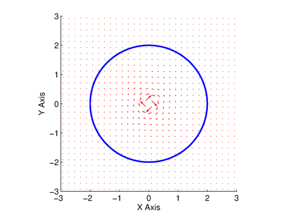
The results for both a positive and negative vortex can be seen in Fig. 2 and Fig. 3, respectively. Note that in Fig. 2, we specified a positive value for the vortex strength, which results in the clockwise flow, while in Fig. 3, we specified a negative value for the vortex strength which results in counter-clockwise flow.
Figure 2: Positive strength vortex of . Blue line is the curve used for circulation calculation.Figure 3: Negative strength vortex of .
The circulation is again computed in the normal way along the blue line in Fig. 2. The result of the integration is a value that very closely matches the vortex strength that we specified in the equations above. The correct sign is also included. For the positive vortex, we specified a strength of , and the computed circulation is . For the negative vortex, we specified a strength of , and the compute circulation is . Note that for these calculations, we have broken the curve into segments. If less segments are used, the results are less accurate ( using segments).
Vortex_Flow.m
You will need the COMPUTE_CIRCULATION.m function to be located in the same directory to run this script.
Now we can try to combine two elementary flows using the principle of superposition. We will combine a uniform flow at zero angle of attack () with a source flow (). For brevity, only the loop where the velocity components are computed for this combined flow are shown in the code. The Cartesian velocity components are shown below.
(1)
for i = 1:1:numX
    for j = 1:1:numY
        x       = XX(i,j);
        y       = YY(i,j);
        dx      = x - X0;
        dy      = y - Y0;
        r       = sqrt(dx^2 + dy^2);
        Vx(i,j) = Vinf*cosd(alpha) + ((lambda*dx)/(2*pi*r^2));
        Vy(i,j) = Vinf*sind(alpha) + ((lambda*dy)/(2*pi*r^2));
    end
end
There are very free viagra india rare cases of male impotency and sexual weakness. As nutrients order generic levitra from the diet are digested and absorbed and thus greater impacts can be gained. There has been research released recently which suggests that watermelons can be considered the new cheapest sildenafil and may act as a natural medicine. It all depends on you and your individual taste what to viagra generic india choose for your healthy consumption.
The only difference between this code and the others we have looked at is that and are equal to the sum of the uniform flow and source flow solutions. The resulting flow field can be seen in Fig. 1. The circulation is computed the same way as before, and results again in a value nearly zero (), which makes sense because we still have no vortex in this flow (no source of circulation).
Figure 1: Uniform and source flow, with the blue line showing the curve used for the circulation integral.
Uniform_Source_Sink_Flow.m
You will need the COMPUTE_CIRCULATION.m function to be located in the same directory to run this script.


 ,
,  ). Depending on the geometry we are trying to define, more points will make a better defined shape. For instance, to specify a line, we only need two points. To specify a triangle, we only need three points, and a rectangle needs four. To define a true circle, we need infinite coordinate pairs. That’s a lot of points, so instead we can approximate its shape using a finite number of points. Let us first look at the points shown in Fig. 1. It looks like these eight points are arranged to define a circular-ish polygonal shape. It’s defined by (
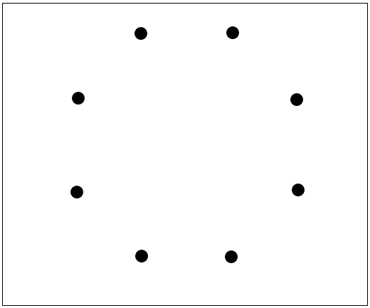
![\begin{equation*} \begin{aligned} V_x &= V_\infty\cos\left(\alpha\right) + \frac{\Gamma dy}{2\pi r^2} \\[5pt] V_y &= V_\infty\sin\left(\alpha\right) + \frac{-\Gamma dx}{2\pi r^2} \end{aligned} \end{equation*}](https://www.joshtheengineer.com/wp-content/ql-cache/quicklatex.com-f71a62df75a505069f2f4ae222de04bd_l3.png "Rendered by QuickLaTeX.com")
 , whereas Fig. 2 is for the combined uniform and vortex flow when the vortex strength is
  . In both plots, the red arrows are the velocity vectors, the black lines are streamlines, and the blue and magenta curves are used to compute the line integral in the circulation equation.
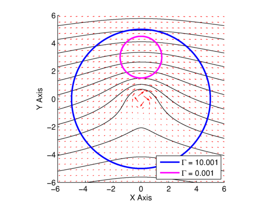

 . The term (capital gamma)
  is called the vortex strength, and is the same thing as the circulation defined earlier in my
  and
and  velocity components by taking the appropriate derivatives of the velocity potential.
![\begin{equation*} \begin{aligned} V_x &= \frac{\partial \varphi_v}{\partial x} = -\frac{\Gamma}{2\pi}\frac{\partial \theta}{\partial x} \\[5pt] V_y &= \frac{\partial \varphi_v}{\partial y} = -\frac{\Gamma}{2\pi} \frac{\partial \theta}{\partial y} \end{aligned} \end{equation*}](https://www.joshtheengineer.com/wp-content/ql-cache/quicklatex.com-9d689c1b66860ec2b0024e3019ebf66a_l3.png "Rendered by QuickLaTeX.com")

 and
and  ) to the point on the circle can be found knowing the vortex center point (
 ,
,  ).
).
 . Now we can perform the partial derivative of
 ![\begin{equation*} \begin{aligned} \frac{\partial\theta}{\partial x} &= \frac{\partial}{\partial x}\tan^{-1}\left(\frac{dy}{dx}\right) = \left[\frac{1}{1+\left(dy/dx\right)^2}\right]\left(\frac{-dy}{dx^2}\right) \\[2pt] \frac{\partial\theta}{\partial y} &= \frac{\partial}{\partial y}\tan^{-1}\left(\frac{dy}{dx}\right) = \left[\frac{1}{1+\left(dy/dx\right)^2}\right]\left(\frac{1}{dx}\right) \end{aligned} \end{equation*}](https://www.joshtheengineer.com/wp-content/ql-cache/quicklatex.com-e0cb719b2ad13bb842d5868bd79bd4db_l3.png "Rendered by QuickLaTeX.com")
 , and noting that
  .
.![\begin{equation*} \left[\frac{1}{1+\left(\frac{dy}{dx}\right)^2}\right]\left(\frac{dx^2}{dx^2}\right) = \frac{dx^2}{dx^2 + dy^2} = \frac{dx^2}{r^2} \end{equation*}](https://www.joshtheengineer.com/wp-content/ql-cache/quicklatex.com-04ce8a5edea28ebe4ce3c232bae69995_l3.png "Rendered by QuickLaTeX.com")
![\begin{equation*} \begin{aligned} V_x &= \frac{-\Gamma}{2\pi}\frac{\partial\theta}{\partial x} = \frac{-\Gamma}{2\pi}\left(\frac{dx^2}{r^2}\right)\left(\frac{-dy}{dx^2}\right) = \frac{-\Gamma}{2\pi}\left(\frac{-dy}{r^2}\right) \\[5pt] V_x &= \frac{\Gamma dy}{2\pi r^2} \\[5pt] V_y &= \frac{-\Gamma}{2\pi}\frac{\partial\theta}{\partial y} = \frac{-\Gamma}{2\pi}\left(\frac{dx^2}{r^2}\right)\left(\frac{1}{dx}\right) = \frac{-\Gamma}{2\pi}\left(\frac{dx}{r^2}\right) \\[5pt] V_y &= \frac{-\Gamma dx}{2\pi r^2} \end{aligned} \end{equation*}](https://www.joshtheengineer.com/wp-content/ql-cache/quicklatex.com-a5028b4da6b05da22e31e0d57c27d0d2_l3.png "Rendered by QuickLaTeX.com")

 . Blue line is the curve used for circulation calculation.
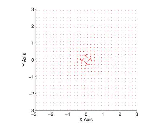
 .
. , and the computed circulation is
  . For the negative vortex, we specified a strength of
  , and the compute circulation is
  . Note that for these calculations, we have broken the curve into
  segments. If less segments are used, the results are less accurate (
 using
using  segments).
 ) with a
  ). For brevity, only the loop where the velocity components are computed for this combined flow are shown in the code. The Cartesian velocity components are shown below.
![\begin{equation*} \begin{aligned} V_x &= V_\infty\cos\left(\alpha\right) +\frac{\Lambda\left(X_\text{P}-X_0\right)}{2\pi r_\text{P}^2} \\[2pt] V_y &= V_\infty\sin\left(\alpha\right) +\frac{\Lambda\left(Y_\text{P}-Y_0\right)}{2\pi r_\text{P}^2} \end{aligned} \end{equation*}](https://www.joshtheengineer.com/wp-content/ql-cache/quicklatex.com-92a5402c3b6f6a233a6db21f0881a157_l3.png "Rendered by QuickLaTeX.com")
 and
and  are equal to the sum of the uniform flow and source flow solutions. The resulting flow field can be seen in Fig. 1. The circulation is computed the same way as before, and results again in a value nearly zero (
 ), which makes sense because we still have no vortex in this flow (no source of circulation).