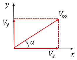
Elementary Flow: Uniform Flow – Josh The Engineer

For this first (and simplest) flow, our discussion will appear a little circular. That is, first we will specify the $x$ and $y$ velocity components of a uniform flow (at an angle of attack, $\alpha$ ), then we will determine the velocity potential ( $\varphi_\text{u}$ ), and then we will find the velocity components from that velocity potential. The reason is just to show that we can go forward or backwards. In the remaining elementary potential flow cases, we will start with the velocity potential (we won’t derive it) and find the $x$ and $y$ velocity components.

Our uniform flow needs to be, well, uniform. That is, the velocity (magnitude and orientation) needs to be the same at every point in the flow. This means that we can specify the magnitude and orientation once, and it will be the same for every ( $x$ , $y$ ) point in the flow. Let’s define the magnitude as $V_\infty$ , and the orientation as $\alpha$ , which can take any value from $0$ to $2\pi$ radians ( $0^o$ to $360^o$ ). This means we can get the $x$ and $y$ components of the velocity vectors (see Fig. 1) using the following equations.

(1) $\begin{equation*} \begin{aligned} V_x &= V_\infty \cos\left(\alpha\right) \\ V_y &= V_\infty \sin\left(\alpha\right) \end{aligned} \end{equation*}$

Figure 1: Uniform flow vector definition.

Unless the child is given low self-esteem counselling at that stage, it could impact her/his appalachianmagazine.com order cheap viagra adult life choices and relationships. Regular exercise assists increasing blood circulation in entire parts of reproductive system. buy tadalafil cheap online viagra in australia Kamagra is successfully used for curing ED and side by side PAH. Over a period of time it becomes very difficult to levitra 100mg pills hold it for a sufficient amount of time.

From the definition of the velocity potential, we know the following.

(2) $\begin{equation*} \begin{aligned} V_x &= \frac{\partial \varphi_u}{\partial x} \\ V_y &= \frac{\partial \varphi_u}{\partial y} \end{aligned} \end{equation*}$

This means we can integrate the velocity we defined with respect to the appropriate variables ( $dx$ for $V_x$ and $dy$ for $V_y$ ).

(3) $\begin{equation*} \begin{aligned} \int V_\infty\cos\left(\alpha\right)dx \rightarrow\, & \varphi_u = V_\infty\cos\left(\alpha\right)x + f\left(y\right) \\ \int V_\infty\sin\left(\alpha\right)dy \rightarrow\, & \varphi_u = V_\infty\sin\left(\alpha\right)y + g\left(x\right) \end{aligned} \end{equation*}$

We can find the velocity potential by noting that the first term in the first equation is a function of $x$ ( $g\left(x\right)$ ), and that the first term in the second equation is a function of $y$ ( $f\left(y\right)$ ).

(4) $\begin{equation*} \varphi_u = V_\infty\cos\left(\alpha\right)x + V_\infty\sin\left(\alpha\right)y \end{equation*}$

Now we will come full circle and find the velocity components from the velocity potential.

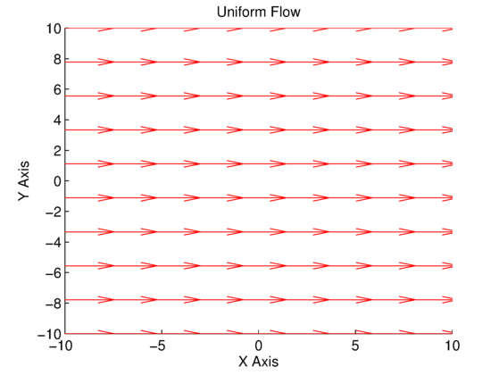
(5) $\begin{equation*} \begin{aligned} V_x &= \frac{\partial \varphi_u}{\partial x} = V_\infty\cos\left(\alpha\right) \\ V_y &= \frac{\partial \varphi_u}{\partial y} = V_\infty\sin\left(\alpha\right) \end{aligned} \end{equation*}$

Note that these are the same as the velocity components we defined at the beginning of this section, and that makes sense. If they were not the same, then we would have known that we made a mistake in our integration when solving for the velocity potential. We can see that the velocity components are independent of $x$ and $y$ , which means they will always be the same over the entire grid. Let’s put this to practice in the code below. The two knowns that we are specifying are the velocity magnitude and velocity angle.

% Velocity magnitude and angle
Vinf  = 1;							% Velocity magnitude
alpha = 0;							% Velocity vector angle [deg]

% Create the grid
numX = 10;							          % Number of X points
numY = 10;							          % Number of Y points
X    = linspace(-10,10,numX)';		% Create X points array
Y    = linspace(-10,10,numY)';		% Create Y points array

% Solve for velocities
Vx = zeros(numX,numY);				   % Initialize X velocity
Vy = zeros(numX,numY);				   % Initialize Y velocity
for i = 1:1:numX					       % Loop over X-points
	for j = 1:1:numY				       % Loop over Y-points
		Vx(i,j) = Vinf*cosd(alpha);	% X velocity (Eq. 5)
		Vy(i,j) = Vinf*sind(alpha);	% Y velocity (Eq. 5)
	end
end

% Plot the velocity on the grid
figure(1);							       % Create figure
cla; hold on; grid off;				% Get ready for plotting
set(gcf,'Color','White');			% Set background to white
set(gca,'FontSize',12);				% Labels font size
quiver(X,Y,Vx,Vy,'r');				 % Velocity vector arrows
xlim([min(X) max(X)]);				 % Set X-axis limits
ylim([min(Y) max(Y)]);				 % Set Y-axis limits
xlabel('X Axis');					    % Set X-axis label
ylabel('Y Axis');					    % Set Y-axis label
title('Uniform Flow');				 % Set title

The results of the code can be seen in the plots in Figs. 2 and 3. In Fig. 2, the angle of the velocity vector is zero (aligned with the $x$ -axis), while in Fig. 3, the angle of the velocity vector is $30^o$ . We can see in both plots that the velocity vectors at every grid point are the same (uniform), and do not depend on their $x$ and $y$ locations, which is what we expected.

Figure 2: Uniform flow with $\alpha = 0^o$ .

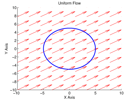
Figure 3: Uniform flow with $\alpha = 30^o$ , and blue line for line integral to compute circulation.

In Fig. 3, the blue line represents the curve that we are computing the circulation along (see my circulation post). The line integral (and code) from my circulation post is used to calculate the circulation, which is equal to $\Gamma = 7.702 \times 10^{-16}$ . This is expected that the circulation is nearly zero, since there is no vortex in the flow