
How do we define a geometric shape, such as a polygon? We define coordinate pairs, such as ( ,
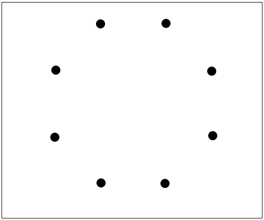
,  ). Depending on the geometry we are trying to define, more points will make a better defined shape. For instance, to specify a line, we only need two points. To specify a triangle, we only need three points, and a rectangle needs four. To define a true circle, we need infinite coordinate pairs. That’s a lot of points, so instead we can approximate its shape using a finite number of points. Let us first look at the points shown in Fig. 1. It looks like these eight points are arranged to define a circular-ish polygonal shape. It’s defined by (, ) pairs, but which point is first, and what order are these points in after the first?
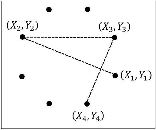
Let us say that the intention was, in fact, to define a circle with eight points. Let’s define the first four points as shown in Fig. 2.
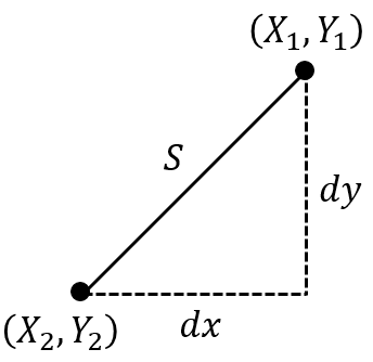
If all you want is to plot the points of a circle, then it’s fine. However, this numbering scheme fails if you want to find the length of the sides of this cicular-ish polygon. This matters for panel method codes where panel length is important, along with panel orientations, etc. The reason this arbitrary numbering scheme fails is because we compute the length of the panel using the two panel endpoints, as shown in Fig. 3.
 .
.The panel length is calculated using the Pythagorean theorem ( ) with slightly different variable names.
(1) 
So now we can see that we need the points in order around the object so that we can approximate the body with panels (Fig. 4a).
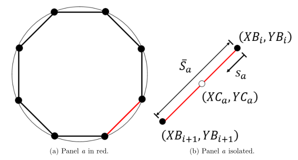
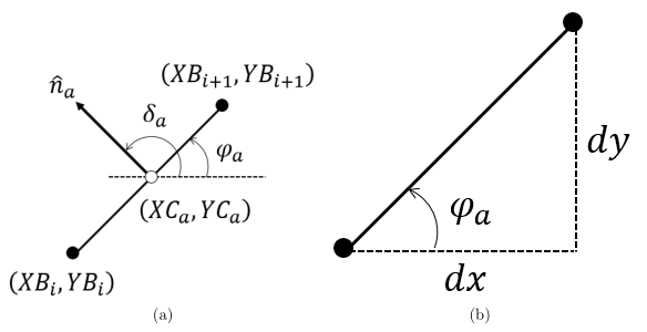
We need some more geometric quantities defined for use in our panel code, so let’s start with some definitions first, and then we will see how we can compute them from our known geometric points. Let’s take just a single panel to simplify things, as shown by the red panel in Fig. 4a. I will call this panel a for the rest of this section, and it is shown with some geometric quantities labeled in Fig. 4b. The descriptions of these geometric quantities can be found in the table below.
| Name | Description |
| Black Dots | Boundary points (B) for panel  |
| White Dot | Control point (C) for panel |
 | Panel length |
 | Distance progress variable along panel |
 | Coordinate of panel control point |
 | Coordinate of panel first boundary point |
 | Coordinate of panel second boundary point |
We can compute the length of the panel with the same equation used previously, with appropriate variables substituted in.
(2) 
We can also easily calculate the control point location using the panel boundary points.
(3) 
For these previous calculations, we could have switched the points  and
and  and nothing would have changed. That is, the values didn’t depend on the orientation of the panel. But now let’s look at the entire circle again. With our initial boundary point numbering (Fig. 5), the panels proceed in a clockwise fashion.
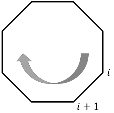 and points labeled, indicating clockwise paneling.
If we had reversed it, then they would have been oriented counter-clockwise. Why is this important? Because we need to define normal and tangential vectors for each panel, that is, the orientations of the panels in space. First, as is usually the case, we define the panel normal vector pointing out of the polygon. This is the same as is done with the conservation equation derivations for example. As we loop around the polygon (panel by panel), we can compute the tangential vectors and normal vectors. For these calculations, I’m going to assume the points are oriented clockwise, then show the calculations, and then show what happens when we use those equations with the orientation reversed.
We’re going to switch over to the top left panel of our circle (Fig. 6a) because it’s the easiest to see what is happening.
There are a couple new variables that need to be defined. In the table below, we can see the rest of the geometric quantities left out of our previous table.
| Name | Description |
 | Angle from positive axis to inside surface of panel |
 | Angle from positive axis to outward normal vector of panel ( ) ) |
 | Angle between freestream vector ( ) and outward normal vector of panel () ) and outward normal vector of panel () |
The control point location and the panel length calculations are the same as calculated previously for the other panel. Now we need the panel angle to the interior, . First we can define  and
and  for the panel.
(4) 
Then we can compute the angle using these two quantities. A schematic of this calculation can be seen in Fig. 6b.
(5) 
To get the value of , all we need to do is add  to . This is always the case; the outward normal for the clockwise definition is always greater than the panel tangential.
(6) 
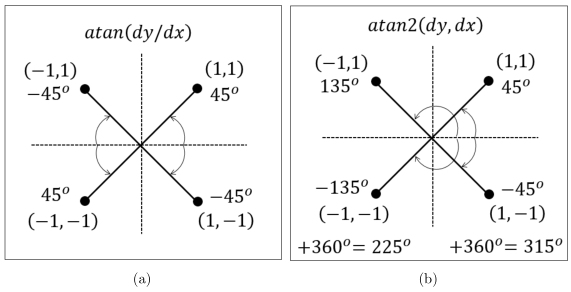
Now, we need to talk about how to compute the inverse tangent on a computer, because it is not trivial. Let’s look at both atan and atan2 functions in each quadrant (Fig. 7a and Fig. 7b, respectively).
 and (b)
  functions.
The atan solutions are non-singular, while the atan2 results are. By “non-singular” I mean that two distinct points can have the same result from the atan function. For example, points  and
and  both result in an angle of
  . The resulting angles using atan2 will always be different for distinct points. We can get the resulting angles from the atan2 to always be positive, and all CCW from horizontal (positive
  -axis) by adding
  to any negative number, as seen in Fig. 7b.
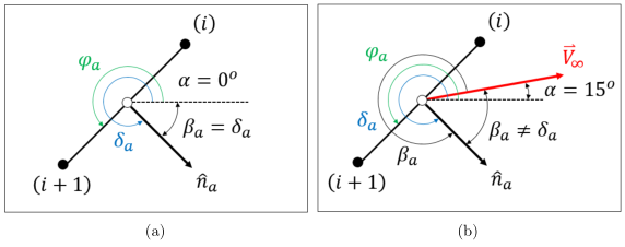
The last geometric issue we need to address is how to include the angle of attack ( ). The angle
  is the angle between the freestream velocity vector () and the panel outward normal vector (), so we use the following equation.
(7) 
Let’s see why this works with an example. first we assume that  (aligned with the -axis) as shown in Fig. 8a. The panel is angle at
  from the -axis, which means the panel orientation angle is
  . The angle of the panel normal is then
  . Finally, we can calculate
  . We can also write this as
  . This is valid because
  and
and  .
.
 and when (b)
  .
.Now let us assume that (no longer aligned with the -axis) as shown in Fig. 8b. The panel is still angled from the -axis, so the panel orientation is still . The angle of the panel normal is also still . Now we can calculated  . We can also write this as
  . This is valid because
  and
and  .
.
Now we will go over to MATLAB to see how to use the information from this section in practice. We will be computing the geometric parameters for both a circle and an airfoil. Let’s start by defining the geometry for a unit circle (radius of unity). A certain  pair is defined solely by the angle as follows.
(8) 
Let’s say that we want to define an eight panel circle. This means that we will need nine boundary points in order to loop all the way around the circle and close the geometry (the first point is the same as the last point). We can use the linspace function in MATLAB to make linearly spaced angles from  to , which will ensure that we get the repeat point at the end because
  . Since we have eight panels, in order to get vertical and horizontal panels, we need to add
  to each of the angles as well.
(9) 
We can the compute the circle boundary points using the relations from above.
(10) 
It was discussed earlier how the orientation of the panels is important (clockwise versus counter-clockwise), so we can add a check in here to make sure they are oriented correctly. If they are oriented in the wrong direction, simply flip the boundary points arrays using the flipud function in MATLAB. We will call this edge orientation variable  . If
. If  then the points are CCW and the arrays are flipped. If
  then the points are CW and we can proceed without any changes in the point arrays.
(11) 
The code for the calculation of the geometric parameters can be seen in the code snippet below. Variables are first initialized, and then each value is calculated for each panel in the for loop. Note that the angle  is computed using the atan2 function (where
  is for calculations in degrees). The addition or subtraction of on lines 14 and 20 are not needed, but are included because they make sure the angles are positive (which is easier to debug if something is wrong).
% Find geometric quantities of airfoil
XC   = zeros(numPan,1);
YC   = zeros(numPan,1);
S    = zeros(numPan,1);
phiD = zeros(numPan,1);
for i = 1:1:numPan
    XC(i)   = 0.5*(XB(i)+XB(i+1));
    YC(i)   = 0.5*(YB(i)+YB(i+1));
    dx      = XB(i+1)-XB(i);
    dy      = YB(i+1)-YB(i);
    S(i)    = (dx^2 + dy^2)^0.5;
    phiD(i) = atan2d(dy,dx);
    if (phiD(i) < 0)
        phiD(i) = phiD(i) + 360;
    end
end

% Compute angle of panel normal w.r.t horizontal and include AoA
betaD              = phiD + 90 - AoA;
betaD(betaD > 360) = betaD(betaD > 360) - 360;
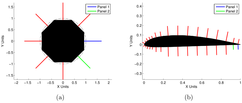
The results of the code for both the circle and an airfoil can be seen in Fig. 9. From these figures, we can see that the panel normal vectors (colored lines) point out of the volume, which is how they are supposed to be oriented based on our definition. The dashed black line in Fig. 9a shows the actual circle that the polygon is approximating.
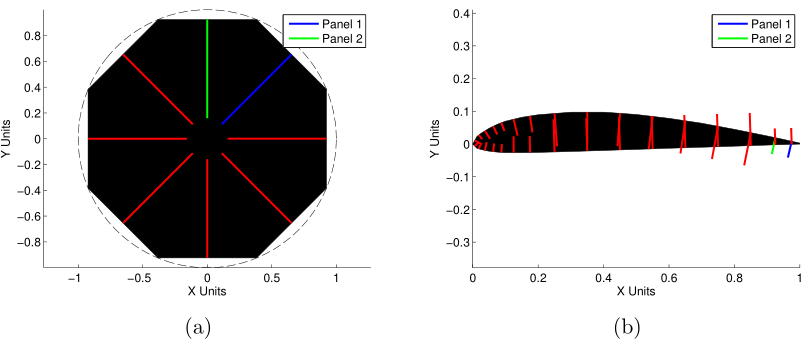
In Fig. 10, we can see what happens when the points are oriented counter-clockwise (visible from orientation of blue and green lines). The panel normal vectors now point into the volume, which will mess with the panel method code we will go through in another post.

If you want to run the airfoil geometry, you will need to download my LOAD_SELIG_AIRFOIL.py code.
Note: I can’t upload “.py” files, so this is a “.txt” file. Just download it and change the extension to “.py”, and it should work fine.
You will need to change the file path on line 36 of the code. This file path should be the directory where all the airfoil DAT files are located.
Note: I can’t upload “.py” files, so this is a “.txt” file. Just download it and change the extension to “.py”, and it should work fine.
If you want to run the airfoil geometry, you will need to download my LOAD_SELIG_AIRFOIL.m code.