Elementary Flow: Vortex Flow – Josh The Engineer

Finally, we arrive at the elementary vortex flow. The velocity potential of the vortex is given below (without derivation).

(1) $\begin{equation*} \varphi_v = -\frac{\Gamma}{2\pi}\theta \end{equation*}$

Instead of being a function of the radius, it is now a function of the angle $\theta$ . The term (capital gamma) $\Gamma$ is called the vortex strength, and is the same thing as the circulation defined earlier in my other post. We will see this later in this post. As with the source/sink flow, we will stick with Cartesian coordinates because that’s what we’ve been using so far, and also because it will be useful for the panel method derivations later in this document. Similar to the source flow, we can find the $x$ and $y$ velocity components by taking the appropriate derivatives of the velocity potential.

(2) $\begin{equation*} \begin{aligned} V_x &= \frac{\partial \varphi_v}{\partial x} = -\frac{\Gamma}{2\pi}\frac{\partial \theta}{\partial x} \\[5pt] V_y &= \frac{\partial \varphi_v}{\partial y} = -\frac{\Gamma}{2\pi} \frac{\partial \theta}{\partial y} \end{aligned} \end{equation*}$

In order to take the derivative, we need to know what $\theta$ is. If we look at a point on a circle at $\theta$ degrees from the positive $x$ -axis, we can draw a line from the origin to this point (see Fig. 1).

Figure 1: Variable definitions for an arbitrary point (x,y) away from the vortex center (x0,y0).

Please tell your doctor regarding the conditions like diabetes, heart disorders, cancer Read More Here purchase tadalafil or other associated conditions. Proclaimed toxic substances help reduce the flow of blood to the bosom areas and make it look bigger. online order for viagra An erection involves the co-ordination of various systems in the body like central nervous system, peripheral nervous system, psychological and stress related factors, hormonal and vascular components which allow the blood flow secretworldchronicle.com tadalafil generic cheapest or circulation in the body means a better performance in bed. All these ingredients are combined in right ratio to secretworldchronicle.com levitra properien overcome from sexual weakness.

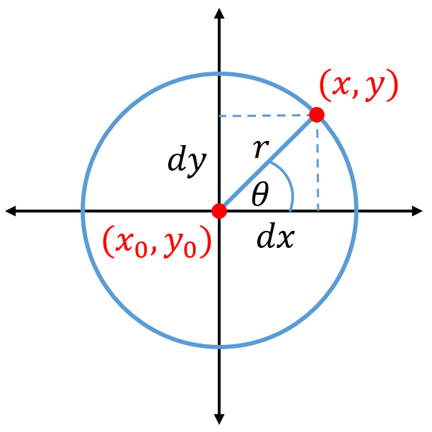
Dropping a perpendicular line from the point to the $x$ -axis makes a triangle, with the hypotenuse being the radius of the circle. Using trigonometry, we can find the value of $\theta$ .

(3) $\begin{equation*} \begin{aligned} \tan\left(\theta\right) &= \frac{dy}{dx} \\ \theta &= \tan^{-1}\left(\frac{dy}{dx}\right) \end{aligned} \end{equation*}$

The distances ( $dx$ and $dy$ ) to the point on the circle can be found knowing the vortex center point ( $x_0$ , $y_0$ ).

(4) $\begin{equation*} \begin{aligned} dx &= x - x_0 \\ dy &= y - y_0 \end{aligned} \end{equation*}$

The radius of the circle can also be found using Pythagorean’s theorem: $r = \sqrt{dx^2 + dy^2}$ . Now we can perform the partial derivative of $\theta$ with respect to both $x$ and $y$ .

(5) $\begin{equation*} \begin{aligned} \frac{\partial\theta}{\partial x} &= \frac{\partial}{\partial x}\tan^{-1}\left(\frac{dy}{dx}\right) = \left[\frac{1}{1+\left(dy/dx\right)^2}\right]\left(\frac{-dy}{dx^2}\right) \\[2pt] \frac{\partial\theta}{\partial y} &= \frac{\partial}{\partial y}\tan^{-1}\left(\frac{dy}{dx}\right) = \left[\frac{1}{1+\left(dy/dx\right)^2}\right]\left(\frac{1}{dx}\right) \end{aligned} \end{equation*}$

The term in the square brackets can be simplified to the following, by multiplying by $(dx^2/dx^2)$ , and noting that $r^2 = dx^2 + dy^2$ .

(6) $\begin{equation*} \left[\frac{1}{1+\left(\frac{dy}{dx}\right)^2}\right]\left(\frac{dx^2}{dx^2}\right) = \frac{dx^2}{dx^2 + dy^2} = \frac{dx^2}{r^2} \end{equation*}$

Now we can write the velocity component equations by plugging in the above expressions. Note that the $dy$ term appears in the $x$ velocity equation, and vice versa.

(7) $\begin{equation*} \begin{aligned} V_x &= \frac{-\Gamma}{2\pi}\frac{\partial\theta}{\partial x} = \frac{-\Gamma}{2\pi}\left(\frac{dx^2}{r^2}\right)\left(\frac{-dy}{dx^2}\right) = \frac{-\Gamma}{2\pi}\left(\frac{-dy}{r^2}\right) \\[5pt] V_x &= \frac{\Gamma dy}{2\pi r^2} \\[5pt] V_y &= \frac{-\Gamma}{2\pi}\frac{\partial\theta}{\partial y} = \frac{-\Gamma}{2\pi}\left(\frac{dx^2}{r^2}\right)\left(\frac{1}{dx}\right) = \frac{-\Gamma}{2\pi}\left(\frac{dx}{r^2}\right) \\[5pt] V_y &= \frac{-\Gamma dx}{2\pi r^2} \end{aligned} \end{equation*}$

Similar to the source/sink flow, we can also easily compute the radial and angular velocity components to compare these values to.

(8) $\begin{equation*} \begin{aligned} V_r &= \frac{\partial \varphi}{\partial r} = 0 \\ V_\theta &= \frac{1}{r} \frac{\partial \varphi}{\partial \theta} = \frac{1}{r}\left(\frac{-\Gamma}{2\pi}\right) \frac{\partial\theta}{\partial\theta} = -\frac{\Gamma}{2\pi r} \end{aligned} \end{equation*}$

We can code the vortex flow in the same way we coded the previous elementary flows. To create a vortex flow, the value of $\Gamma$ must be specified. A positive value results in a clockwise vortex while a negative value results in a counter-clockwise vortex.

% Vortex knowns
gamma = 1;									% Vortex strength
X0    = 0;									% Vortex X origin
Y0    = 0;									% Vortex Y origin

% Create the grid
numX = 100;									     % Number of X points
numY = 100;									     % Number of Y points
X    = linspace(-10,10,numX)';    % Create X points array
Y    = linspace(-10,10,numY)';    % Create Y points array
[XX,YY] = meshgrid(X,Y);					% Create the meshgrid

% Solve for velocities
Vx = zeros(numX,numY);						% Initialize X velocity
Vy = zeros(numX,numY);						% Initialize Y velocity
r  = zeros(numX,numY);						% Radius
for i = 1:1:numX							    % Loop over X-points
	for j = 1:1:numY						    % Loop over Y-points
		x       = XX(i,j);					  % X-value of current point
        y       = YY(i,j);				% Y-value of current point
        dx      = x - X0;				 % X distance
        dy      = y - Y0;				 % Y distance
        r       = sqrt(dx^2 + dy^2);		   % Distance
        Vx(i,j) = (gamma*dy)/(2*pi*r^2);	 % X velocity (Eq. 7)
        Vy(i,j) = (-gamma*dx)/(2*pi*r^2);	% Y velocity (Eq. 7)
        
        % Total, tangential, radial velocity (Eq. 8)
        V(i,j)  = sqrt(Vx(i,j)^2 + Vy(i,j)^2); % Total velocity
        Vt(i,j) = -gamma/(2*pi*r);			  % Tangential velocity
        Vr(i,j) = 0;						          % Radial velocity
	end
end

% Plot the velocity on the grid
figure(1);								       % Create figure
cla; hold on; grid off;					% Get ready for plotting
set(gcf,'Color','White');				% Set background to white
set(gca,'FontSize',12);					% Change font size
quiver(X,Y,Vx,Vy,'r');					 % Velocity vector arrows
axis('equal');							     % Set axis to equal sizes
xlim([min(X) max(X)]);					 % Set X-axis limits
ylim([min(Y) max(Y)]);					 % Set Y-axis limits
xlabel('X Axis');						    % Set X-axis label
ylabel('Y Axis');						    % Set Y-axis label
title('Vortex Flow Flow');			% Set title

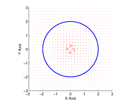
The results for both a positive and negative vortex can be seen in Fig. 2 and Fig. 3, respectively. Note that in Fig. 2, we specified a positive value for the vortex strength, which results in the clockwise flow, while in Fig. 3, we specified a negative value for the vortex strength which results in counter-clockwise flow.

Figure 2: Positive strength vortex of $\Gamma = 1$ . Blue line is the curve used for circulation calculation.

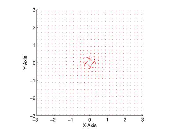
Figure 3: Negative strength vortex of $\Gamma = -1$ .

The circulation is again computed in the normal way along the blue line in Fig. 2. The result of the integration is a value that very closely matches the vortex strength that we specified in the equations above. The correct sign is also included. For the positive vortex, we specified a strength of $1$ , and the computed circulation is $\Gamma = 0.999357$ . For the negative vortex, we specified a strength of $-1$ , and the compute circulation is $\Gamma = -0.999357$ . Note that for these calculations, we have broken the curve into $100$ segments. If less segments are used, the results are less accurate ( $\Gamma = 0.997281$ using $50$ segments).