In my previous post on uniform flow, we saw how we can use the velocity potential to find the velocity component of the flow at discrete grid points. We will use this methodology again here to find the velocity induced at discrete grid points from a source/sink in the flow. The velocity of source/sink flow is given below (with no derivation here).
(1) 
We can see that the velocity potential is a function of the radial distance from the origin of the source ( ), and so most textbooks will solve for the radial and angular components of the velocity (
 and
and  ). We will stick with the Cartesian coordinates here though, because it will show another method and it will also be helpful in later derivations of the source panel method (SPM) and vortex panel method (VPM). The source strength (uppercase lambda),
  , is constant here, so we can take it out of the derivative term.
(2) ![\begin{equation*} \begin{aligned} V_x &= \frac{\partial \varphi_s}{\partial x} = \frac{\Lambda}{2\pi}\frac{\partial \text{ln}\left(r\right)}{\partial x} = \frac{\Lambda}{2\pi r} \frac{\partial r}{\partial x} \\[5pt] V_y &= \frac{\partial \varphi_s}{\partial y} = \frac{\Lambda}{2\pi}\frac{\partial \text{ln}\left(r\right)}{\partial y} = \frac{\Lambda}{2\pi r} \frac{\partial r}{\partial y} \end{aligned} \end{equation*}](https://www.joshtheengineer.com/wp-content/ql-cache/quicklatex.com-904cf085c91be88c03a2a49bd27e7825_l3.png "Rendered by QuickLaTeX.com")
The velocity induced at point  (
( ,
,  ) depends on the distance from the sourse/sink origin (
 ,
,  ),
),  , which is defined below.
(3) 
Performing the derivative using the chain rule, we get the following expression for the partial derivatives.
(4) ![\begin{equation*} \begin{aligned} \frac{\partial r_\text{P}}{\partial x} &= \frac{1}{2}\left[\left(X_\text{P}-X_0\right)^2 + \left(Y_\text{P}-Y_0\right)^2\right]^{-1/2}\left(2\right)\left(X_\text{P}-X_0\right) \\[2pt] &= \frac{\left(X_\text{P}-X_0\right)}{r_\text{P}} \\[2pt] \frac{\partial r_\text{P}}{\partial y} &= \frac{1}{2}\left[\left(X_\text{P}-X_0\right)^2 + \left(Y_\text{P}-Y_0\right)^2\right]^{-1/2}\left(2\right)\left(Y_\text{P}-Y_0\right)\\[2pt] &= \frac{\left(Y_\text{P}-Y_0\right)}{r_\text{P}} \end{aligned} \end{equation*}](https://www.joshtheengineer.com/wp-content/ql-cache/quicklatex.com-4b20d0f8c14c3eb35d5073440ed7edea_l3.png "Rendered by QuickLaTeX.com")
Plugging these expressions into the  and
and  equations from Eq. 2, we obtain the following.
(5) ![\begin{equation*} \begin{aligned} V_x &= \frac{\Lambda \left(X_\text{P}-X_0\right)}{2\pi r_\text{P}^2} \\[2pt] V_y &= \frac{\Lambda \left(Y_\text{P}-Y_0\right)}{2\pi r_\text{P}^2} \end{aligned} \end{equation*}](https://www.joshtheengineer.com/wp-content/ql-cache/quicklatex.com-9c2bbfd92597c723d91ebf6b18c32914_l3.png "Rendered by QuickLaTeX.com")
We can code the source/sink flow in the same way we coded the uniform flow. Note that in Python, lambda is a reserved keyword that is used to create an anonymous function, so I have used lmbda instead in my Python code. To create a source flow, the value of must be positive, while for sink flow is negative.
% Source/sink knowns
lambda = 1;									 % Source/sink magnitude
X0     = 0;									 % Source/sink X origin
Y0     = 0;									 % Source/sink Y origin

% Create the grid
numX = 20;                        % Number of X points
numY = 20;	                      % Number of Y points
X    = linspace(-10,10,numX)';		% Create X points array
Y    = linspace(-10,10,numY)';		% Create Y points array
[XX,YY] = meshgrid(X,Y);					% Create the meshgrid

% Solve for velocities
Vx = zeros(numX,numY);			    % Initialize X velocity
Vy = zeros(numX,numY);			    % Initialize Y velocity
for i = 1:1:numX							  % Loop over X-points
	for j = 1:1:numY						  % Loop over Y-points
		x  = XX(i,j);						   % X-value of current point
		y  = YY(i,j);						   % Y-value of current point
		dx = x - X0;						    % X distance
		dy = y - Y0;						    % Y distance
		r  = sqrt(dx^2 + dy^2);				     % Distance (Eq. 3)
		Vx(i,j) = (lambda*dx)/(2*pi*r^2);	 % X velocity (Eq. 4)
		Vy(i,j) = (lambda*dy)/(2*pi*r^2);	 % Y velocity (Eq. 4)

		V(i,j)  = sqrt(Vx(i,j)^2+Vy(i,j)^2); % Total velocity
		Vr(i,j) = lambda/(2*pi*r);			     % Radial velocity
	end
end

% Plot the velocity on the grid
figure(1);									   % Create figure
cla; hold on; grid off;		    % Get ready for plotting
set(gcf,'Color','White');	    % Set background to white
set(gca,'FontSize',12);		    % Change font size
quiver(X,Y,Vx,Vy,'r');			   % Velocity vector arrows
xlim([min(X) max(X)]);			   % Set X-axis limits
ylim([min(Y) max(Y)]);			   % Set Y-axis limits
xlabel('X Axis');							% Set X-axis label
ylabel('Y Axis');							% Set Y-axis label
title('Source/Sink Flow');		 % Set title
Since the source and sink flow is usually described by the radial and angular components, let’s compute their velocities below ( computed on line 27 in the code).
(6) 
Since the angular component of the velocity is zero, we can compare the magnitude of the radial component to the magnitude of the velocity from the Cartesian and components. In the code (line 26), the Cartesian velocity magnitude is  . Comparing these two matrices, it is clear that they are the same, which is a good check that our Cartesian velocity derivation is correct.
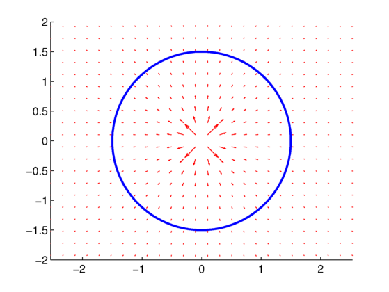
The results for source and sink flow can be seen in Fig. 1 and Fig. 2, respectively. The velocity vector arrows either point directly out from the origin (source) or directly into the origin (sink).
 . Blue line is curve along which the circulation is calculated
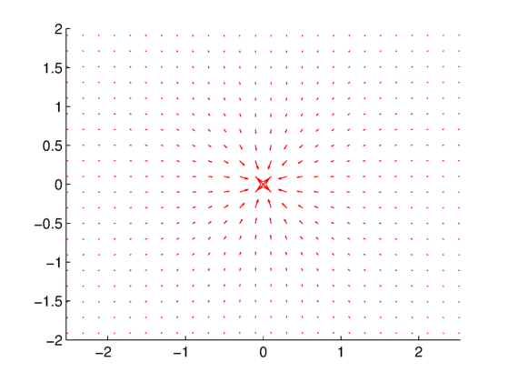
 .
.We can also now compute the circulation around the solid blue curve as shown in Fig. 1. Again, the expected circulation is zero since there is no vortex in the flow, and this agrees with the computed circulation of  . The same circulation can be computed for the sink in Fig. 2, and the same results are obtained.
You will need the COMPUTE_CIRCULATION.m function file in the same folder in order to run this code.

You will need the COMPUTE_CIRCULATION.py function file in the same folder in order to run this code.
Note: I can’t upload “.py” files, so this is a “.txt” file. Just download it and change the extension to “.py”, and it should work fine.
Note: I can’t upload “.py” files, so this is a “.txt” file. Just download it and change the extension to “.py”, and it should work fine.
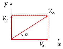
 and
and  velocity components of a uniform flow (at an angle of attack,
  ), then we will determine the velocity potential (
 ), and then we will find the velocity components from that velocity potential. The reason is just to show that we can go forward or backwards. In the remaining elementary potential flow cases, we will start with the velocity potential (we won’t derive it) and find the
  , and the orientation as
  to
to  radians (
 to
to  ). This means we can get the

 for
for  for
for 
 ), and that the first term in the second equation is a function of
  ).
).

 . We can see in both plots that the velocity vectors at every grid point are the same (uniform), and do not depend on their
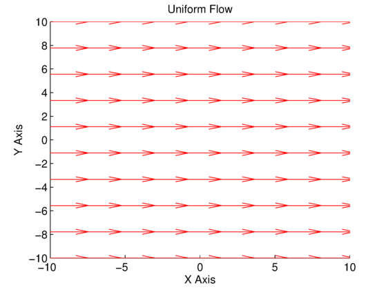
 .
.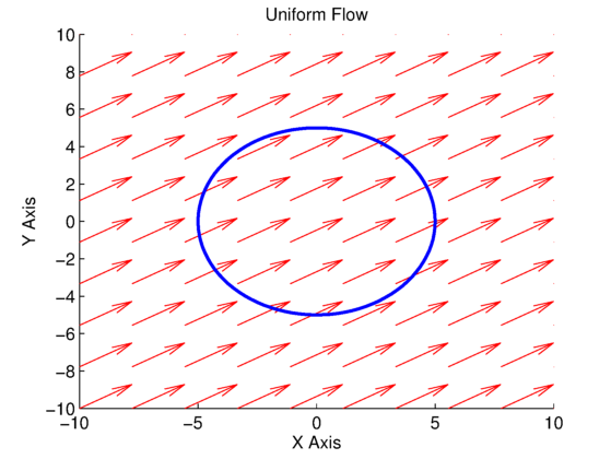
 , and blue line for line integral to compute circulation.
 . This is expected that the circulation is nearly zero, since there is no vortex in the flow